Polynomial Mathematical Operations
API Keywords: polynomial math
A number of liquid modules require polynomial manipulations, particularly those involving filter design where transfer functions are represented as the explicit ratio of polynomials in \(z^{-1}\) . This sub-module is not intended to be complete, but rather is required for the proper functionality of other modules. Like matrices, polynomials in liquid do not use a particular data type, but are stored as memory arrays.
$$ P_n(x) = \sum_{k=0}^{n}{c_k x^k} = c_0 + c_1 x + c_2 x^2 + \cdots + c_n x^n $$An \(n^{th}\) -order polynomial has \(n+1\) coefficients ordered in memory in increasing degree.
.. footnote
Note that this convention is reversed from that used in
{link:http://www.gnu.org/software/octave/web}{Octave}.
For example, a \(2^{nd}\) -order polynomial \(0.1 -2.4x + 1.3x^2\) stored in an array float c[] has c[0]=0.1 , c[1]=-2.4 , and c[2]=1.3 .
Notice that all routines for the type float are prefaced with polyf . This follows the naming convention of the standard C library routines which append an f to the end of methods operating on floating-point precision types. Similar matrix interfaces exist in liquid for double ( poly ), double complex ( polyc ), and float complex ( polycf ).
polyf_val()∞
The polyf_val(*p,k,x) method evaluates the polynomial \(P_n(x)\) at\(x_0\) where the k coefficients are stored in the input array p . Here is a brief example which evaluates \(P_2(x) = 0.2 + 1.0x + 0.4x^2\) at \(x=1.3\) :
float p[3] = {0.2f, 1.0f, 0.4f};
float x = 1.3f;
float y = polyf_val(p,3,x);
>> y = 2.17599988
polyf_fit()∞
The polyf_fit(*x,*y,n,*p,k) method fits data to a polynomial of order \(k-1\) from \(n\) samples using the least-squares method on the input data vectors\(\vec{x}=[x_0,x_1,\cdots,x_{n-1}]^T\) and\(\vec{y}=[y_0,y_1,\cdots,y_{n-1}]^T\) . Internally liquid uses matrix algebra to solve the system of equations
$$ \vec{p} = \left(\vec{X}^T\vec{X}\right)^{-1}\vec{X}^T\vec{y} $$where
$$ \vec{X} = \begin{bmatrix} 1 & x_0 & x_0^2 & \cdots & x_0^{k} \\ 1 & x_1 & x_1^2 & \cdots & x_1^{k} \\ \\ 1 & x_{n-1} & x_{n-1}^2 & \cdots & x_{n-1}^{k} \end{bmatrix} $$For example this script fits the 4 data samples to a linear (first-order, two coefficients) polynomial:
float x[4] = {0.0f,  1.0f,  2.0f,  3.0f};
float y[4] = {0.85f, 3.07f, 5.07f, 7.16f};
float p[2];
polyf_fit(x,y,4,p,2);
>> p = { 0.89800072, 2.09299946}
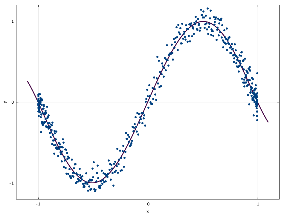
Figure [fig-polyfit]. polyf_fit example
polyf_fit_lagrange()∞
The polyf_fit_lagrange(*x,*y,n,*p) method fit a dataset of \(n\) sample points to exact polynomial of order \(n-1\) using Lagrange interpolation. Given input vectors\(\vec{x}=[x_0,x_1,\cdots,x_{n-1}]^T\) and\(\vec{y}=[y_0,y_1,\cdots,y_{n-1}]^T\) , the interpolating polynomial is
$$ P_{n-1}(x) = \sum_{j=0}^{n-1} { \left[ y_j \prod_{{k=0}\atop{k \ne j}}^{n-1} { \frac{x-x_k}{x_j-x_k} } \right] } $$For example this script fits the 4 data samples to a cubic (third-order, four coefficients) polynomial:
float x[4] = {0.0f,  1.0f,  2.0f,  3.0f};
float y[4] = {0.85f, 3.07f, 5.07f, 7.16f};
float p[4];
polyf_fit_lagrange(x,y,4,p);
>> p = { 0.85000002, 2.43333268, -0.26499939, 0.05166650}
Notice that polyf_fit_lagrange(x,y,n,p) is mathematically equivalent to polyf_fit(x,y,n,p,n) , but is computed in fewer steps. See also polyf_expandroots .
polyf_interp_lagrange()∞
The polyf_interp_lagrange(*x,*y,n,x0) method uses Lagrange polynomials to find the interpolant\((\dot{x},\dot{y})\) from a set of \(n\) pairs\(\vec{x}=[x_0,x_1,\cdots,x_{n-1}]^T\) and\(\vec{y}=[y_0,y_1,\cdots,y_{n-1}]^T\) .
$$ \dot{y} = \sum_{j=0}^{n-1} { \left[ y_j \prod_{{k=0}\atop{k \ne j}}^{n-1} { \frac{\dot{x}-x_k}{x_j-x_k} } \right] } $$For example this script interpolates between the 4 data points
float x[4] = {0.0f,  1.0f,  2.0f,  3.0f};
float y[4] = {0.85f, 3.07f, 5.07f, 7.16f};
float x0 = 0.5f;
float y0 = polyf_interp_lagrange(x,y,4,x0);
>> y0 = 2.00687504
See also polyf_fit_lagrange() .
polyf_fit_lagrange_barycentric()∞
The polyf_fit_lagrange_barycentric(*x,n,*w) method computes the barycentric weights \(\vec{w}\) of \(\vec{x}\) via
$$ w_j = \frac{1}{ \prod_{k \ne j}{\left(x_j - x_k\right)} } $$which can be used to compute the interpolant \((\dot{x},\dot{y})\) with fewer computations.
float x[4] = {0.0f,  1.0f,  2.0f,  3.0f};
float w[4];
polyf_fit_lagrange_barycentric(x,4,w);
>> w = { 1.00000000, -3.00000000, 3.00000000, -1.00000000}
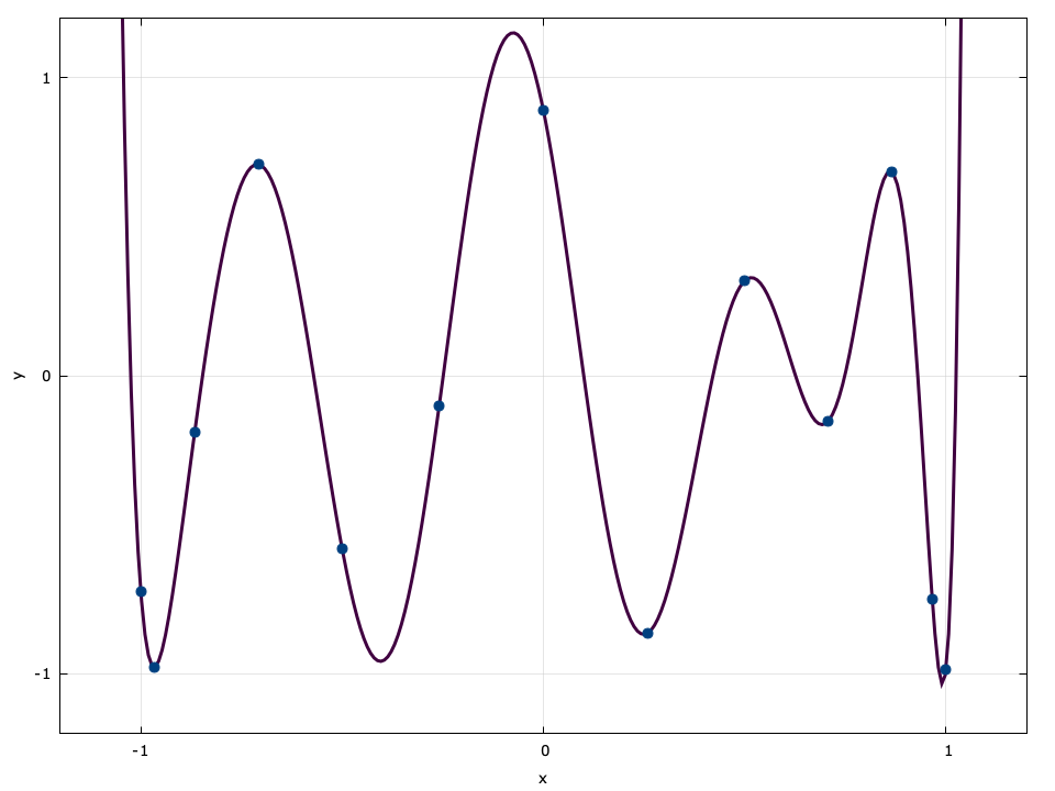
Figure [fig-polyfit_lagrange]. polyf_fit_lagrange_barycentric example
.. input doc/latex.gen/math_polyfit_lagrange.tex
polyf_val_lagrange_barycentric()∞
The polyf_val_lagrange_barycentric(*x,*y,*w,x0,n) method computes the interpolant \((\dot{x},\dot{y})\) given the barycentric weights \(\vec{w}\) (defined above) as
$$ \dot{y} = \frac{ \sum\limits_{j=0}^{k-1}{ w_j y_j /(\dot{x}-x_j) } } { \sum\limits_{j=0}^{k-1}{ w_j /(\dot{x}-x_j) } } $$This is the preferred method for computing Lagrange interpolating polynomials, particularly if \(\vec{x}\) is unchanging. The function returns \(\dot{y}\) if \(\dot{x}\) is equal to any \(x_j\) .
float x[4] = {0.0f,  1.0f,  2.0f,  3.0f};
float y[4] = {0.85f, 3.07f, 5.07f, 7.16f};
float w[4];
polyf_fit_lagrange_barycentric(x,4,w);
float x0 = 0.5f;
float y0 = polyf_val_lagrange_barycentric(x,y,w,x0,4);
>> y0 = 2.00687504
Lagrange polynomials of the barycentric form are used heavily in liquid 's implementation of the Parks-McClellan algorithm ( firdespm ) for filter design (see [ref:section-filter-firdespm] ).
polyf_expandbinomial()∞
The polyf_expandbinomial(n,*p) method expands the a polynomial as a binomial series
$$ P_n(x) = (x+1)^n = \sum_{k=0}^{n}{ {n \choose k} x^k} $$For example the following script will compute\(P_3(x) = (1+x)^3\) :
float p[4];
polyf_expandbinomial(3,p);
>> p = { 1.00000000, 3.00000000, 3.00000000, 1.00000000}
polyf_expandbinomial_pm()∞
Expands the a polynomial as an alternating binomial series
$$ P_n(x) = (x+1)^m (x-1)^{n-m} = \left\{ \sum_{k=0}^{m} { {n \choose k} x^k} \right\} \left\{ \sum_{k=0}^{n-m}{ {n \choose k} (-x)^k} \right\} $$For example the following script will compute\(P_3(x) = (1+x)^2(1-x)\) :
float p[4];
polyf_expandbinomial_pm(2,1,p);
>> p = { 1.00000000, 1.00000000, -1.00000000, -1.00000000}
polyf_expandroots()∞
The polyf_expandroots(*r,n,*p) method expands the a polynomial based on its roots
$$ P_n(x) = \prod_{k=0}^{n-1}{(x - r_k)} $$where \(r_k\) are the roots of \(P_n(x)\) . For example, this script will expand the polynomial\(P_3(x) = (x-1)(x+2)(x-3)\) which has roots\(\{1,-2,3\}\) :
float roots[3] = {1.0f, -2.0f, 3.0f};
float p[4];
polyf_expandroots(roots,3,p);
>> p = { 6.00000000, -5.00000000, -2.00000000, 1.00000000}
polyf_expandroots2()∞
The polyf_expandroots2(*a,*b,n,*p) method expands the a polynomial as
$$ P_n(x) = \prod_{k=0}^{n-1}{(b_kx-a_k)} $$by first factoring out the \(b_k\) terms, invoking polyf_expandroots() , and multiplying the result by \(\prod_k{b_k}\) . For example, this script will expand the polynomial\(P_3(x) = (2x-1)(-3x+2)(-x-3)\) :
float b[3] = { 2.0f, -3.0f, -1.0f};
float a[3] = { 1.0f, -2.0f,  3.0f};
float p[4];
polyf_expandroots2(b,a,3,p);
>> p = { 6.00000000, 11.00000000, -19.00000000, 6.00000000}
polyf_findroots()∞
The polyf_findroots(*p,n,*r) method finds the \(n\) roots of the \(n^{th}\) -order polynomial using Bairstow's method. For an \(n^{th}\) -order polynomial \(P_n(x)\) given by
$$ P_n(x) = \prod_{k=0}^{n-1}{(x-r_k)} $$there exists at least one quadratic polynomial \(p_{2}(x)=u + vx + x^2\) which exactly divides \(P_{n}(x)\) and has two roots (possibly complex)
$$ r_0 = \frac{1}{2}\left(-v-\sqrt{v^2-4u}\right), \; \\ r_1 = \frac{1}{2}\left(-v+\sqrt{v^2-4u}\right) $$If indeed the roots \(r_0\) and \(r_1\) are complex, they are also complex conjugates. Bairstow's method uses Newtonian iterations to find a pair \(u\) and \(v\) which are both finite and real-valued. This method has several advantages over other methods
- iterations operate on real-valued math, even if the roots are complex
- the algorithm is capable of handling multiple roots (unlike the Durand-Kerner method), i.e. \(P_{n}(x) = (x-2)(x-2)(x-2)\cdots\)
- the algorithm does not rely on expanding the full polynomial and is therefore resilient to machine precision
Each iteration of Bairstow's algorithm reduces the original polynomial order by two, eventually collapsing the polynomial. The initial choice of \(u\) and \(v\) determine both algorithm convergence and speed.
liquid implements Bairstow's method with the polyf_findroots() function which accepts an \(n^{th}\) -order polynomial in standard expanded form and computes its \(n\) roots. The last term of the polynomial (highest order) cannot be zero, otherwise the algorithm will not converge.
polyf_mul()∞
The polyf_mul(*P,n,*Q,m,*S) method multiplies two polynomials \(P_n(x)\) and \(Q_m(x)\) to produce the resulting polynomial \(S_{n+m-1}(x)\) .