Linear Modem Bit Error Rates, Part I: Simulation
By  on February 5, 2015
Keywords: modulation modem bit error rate BER simulation
In this two-part tutorial I describe how to derive and simulate bit error rates for several linear modulation schemes using the C programming language. Part I of this tutorial explains how to simulate bit error rates for linear modulation schemes using the C programming language and [ref:liquid-dsp] . Part II derives the theoretical bit error rates values for several common modulation types. You can download a tarball of the source code to generate this example here: liquid_modem_ber_example.tar.gz .
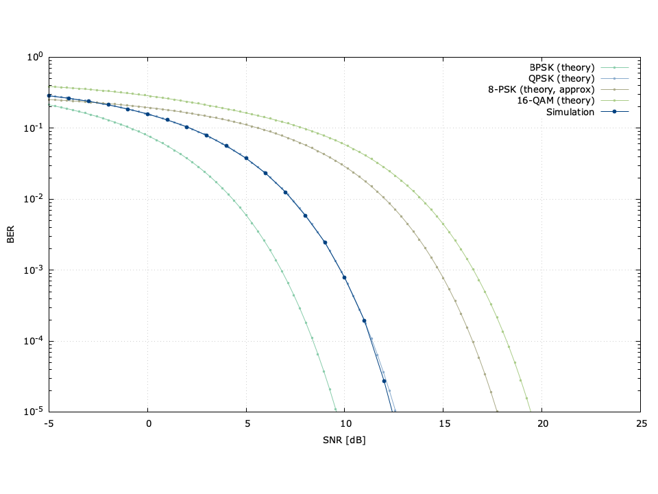
Figure [modem_ber_example]. Digital linear modem bit error rate demonstration. The simulated curve is using QPSK.
Before You Begin...∞
For this example, you will need on your local machine:
- a text editor such as Vim
- a C compiler such as gcc .
- a copy of liquid-dsp installed
- a copy of Gnuplot or Octave for generating figures
- a terminal
The source code is provided up front in a single file with a full description of its operation. Once compiled, the program will run a simulation of the linear modulator/demodulator in an additive white noise channel, generating a data file which can be plotted using either Gnuplot or Octave . The problem statement and a brief theoretical description of linear modulation is given in the next section. A walk-through of the source code follows.
// https://liquidsdr.org/blog/modem-ber-sim : simulate modem bit error rate
#include <stdio.h>
#include <stdlib.h>
#include <complex.h>
#include <math.h>
#include <liquid/liquid.h>

int main() {
    // simulation parameters
    modulation_scheme ms    = LIQUID_MODEM_QPSK; // modulation scheme
    float SNRdB_min         = -5.0f;             // starting SNR value
    float SNRdB_max         = 30.0f;             // ending SNR value
    float SNRdB_step        =  1.0f;             // step size
    unsigned int num_trials = 1e6;               // number of symbols

    // create modem objects
    modem mod = modem_create(ms);   // modulator
    modem dem = modem_create(ms);   // demodulator

    // compute derived values and initialize counters
    unsigned int  m = modem_get_bps(mod);       // modulation bits/symbol
    unsigned int  M = 1 << m;                   // constellation size: 2^m
    unsigned int  i, sym_in, sym_out;
    float complex sample;

    // iterate through SNR values
    printf("# modulation scheme : %s\n", modulation_types[ms].name);
    printf("# %8s %8s %8s %12s\n", "SNR [dB]", "errors", "trials", "BER");
    float SNRdB = SNRdB_min;    // set SNR value
    while (1) {
        // compute noise standard deviation
        float nstd = powf(10.0f, -SNRdB/20.0f);

        // reset modem objects (only necessary for differential schemes)
        modem_reset(mod);
        modem_reset(dem);

        // run trials
        unsigned int num_bit_errors = 0;
        for (i=0; i<num_trials; i++) {
            // generate random input symbol and modulate
            sym_in = rand() % M;
            modem_modulate(mod, sym_in, &sample);

            // add complex noise and demodulate
            sample += nstd*(randnf() + _Complex_I*randnf())/sqrtf(2.0f);
            modem_demodulate(dem, sample, &sym_out);

            // count errors
            num_bit_errors += count_bit_errors(sym_in, sym_out);
        }

        // compute results and print formatted results to screen
        unsigned int num_bit_trials = m * num_trials;
        float ber = (float)num_bit_errors / (float)(num_bit_trials);
        printf("  %8.2f %8u %8u %12.4e\n", SNRdB, num_bit_errors, num_bit_trials, ber);

        // stop iterating if SNR exceed maximum or no errors were detected
        SNRdB += SNRdB_step;
        if (SNRdB > SNRdB_max || num_bit_errors == 0)
            break;
    }

    // destroy modem objects and return
    modem_destroy(mod);
    modem_destroy(dem);
    return 0;
}
Problem Statement∞
Digital communications systems convey information bits by modulating the time-varying characteristics of a sinusoid (the "carrier") to represent a discrete set of messages. The discrete alphabet of symbols generally represents a sequence of bits. The receiver simply needs to make a decision about which symbol was transmitted to recover the information. In practice it is almost certain that the received sample won't match the transmitted symbol exactly. This is generally due to noise and distortion, often realized through inter-symbol interference, an artifact of a imperfect filtering. However, provided that the noise and distortion is sufficiently small, digital systems have the ability to perfectly reconstruct the transmitted message at the receiver. This is not possible with analog communications, and is one of the reasons why digital communications are so prevalent in modern systems.
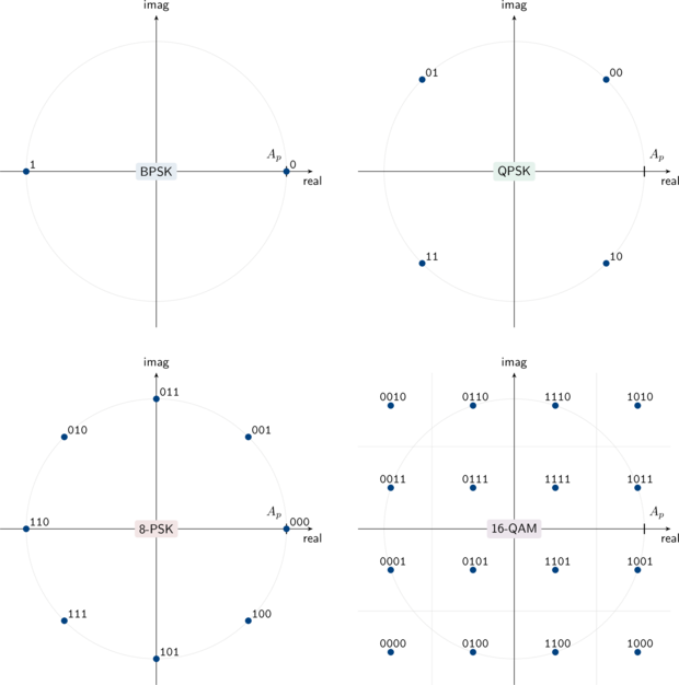
Figure [constellations]. Common linear digital modulation schemes with an average pulse amlitude \(A_p\)
For simplicity let's confine the discussion to linear modulation schemes: those whose resulting transmitted signal is simply a linear combination of data symbols and filter pulses. Figure [ref:constellations] above depicts the constellation diagram of some common linear digital modulation schemes used in modern communications systems with an average pulse amplitude \(A_p\) . Note that each point on the constellation represents a unique set of bits. Given an information message \(k \in \{0,1,\ldots,M-1\}\) , the transmitted symbol at complex baseband is the complex value \(s_k\) in the set \(\mathcal{S}_M = \{s_0,s_1,\ldots,s_{M-1}\}\) . For instance, if the information message is \(k=2\) for quadrature phase-shift keying, ( 10 binary), then \(s_2 = (1 - j)A_p/\sqrt{2}\) according to [ref:constellation_qpsk] . Assuming perfect timing and carrier recovery the received sample will typically be the transmitted symbol with additional noise:
$$ r = s_k + n $$Under typical situations (the noise is uncorrelated, all symbols are equally likely to be used, etc.) the receiver's best guess at the transmitted symbol will be the one which is closest to the received sample. That is, linear modems demodulate by finding the closest of \(M\) symbols in the set \(\mathcal{S}_M\) to the received symbol \(r\) , viz
$$ \hat{s}_k = \underset{s_k \in \mathcal{S}_M}{\arg\min} \bigl\{ \| r - s_k \| \bigr\} $$For example, if the received sample \(r\) falls in the lower right quadrant in [ref:constellation_qpsk] the receiver will assume the transmitted symbol was\(s_2\) and that the message was 10 .
Getting the Source Code∞
You can download the source code for this simulation by clicking the link provided at the top of this page. The compressed archive contains the following files:
- modem_ber_example.c : the source code for the simulation
- modem_ber_example.gnuplot : a Gnuplot script to convert the results of the simulation into a figure
- modem_ber_example.m : an Octave/MATLAB script as an alternative to Gnuplot for generating a figure
- makefile : a make script to automatically build and run the simulation, and generate a plot of the results
Unzip the tarball, move into the directory, and then build the example
$ tar -xvf liquid_modem_ber_example.tar.gz
$ cd liquid_modem_ber_example/
$ make
If successful, the make command will compile the program, execute it while piping the results to modem_ber_example.dat , and then run gnuplot to create an image file modem_ber_example.png similar to Figure [ref:modem_ber_example] at the top of this page.
Source Code Breakdown∞
The program initially sets the parameters for the simulation, including the modulation scheme (QPSK in this case) as well as the range of signal-to-noise ratios and the number of symbol trials to test. Symbols are generated one at a time in the main loop with noise added and the resulting bit errors on the demodulator output are counted. The loop breaks when either the maximum SNR is reached or no bit errors were encountered. Note that because the simulation runs one million symbols for each SNR step, (that's two million bits for QPSK) the simulation might take a few seconds, depending upon the speed of your machine. There are certainly more sophisticated methods for sweeping bit error-rate curves. For example, it's usually only necessary to observe a certain number of bit errors rather than a total number of bits. The program produces an output file that should contain data that looks something like this:
# modulation scheme : qpsk
# SNR [dB]   errors   trials          BER
     -5.00   574017  2000000   2.8701e-01
     -4.00   528628  2000000   2.6431e-01
     -3.00   479644  2000000   2.3982e-01
     -2.00   427648  2000000   2.1382e-01
     -1.00   372221  2000000   1.8611e-01
      0.00   317577  2000000   1.5879e-01
      1.00   261596  2000000   1.3080e-01
      2.00   208781  2000000   1.0439e-01
      3.00   158412  2000000   7.9206e-02
      4.00   112225  2000000   5.6113e-02
      5.00    75365  2000000   3.7682e-02
      6.00    46063  2000000   2.3031e-02
      7.00    25210  2000000   1.2605e-02
      8.00    11804  2000000   5.9020e-03
      9.00     4932  2000000   2.4660e-03
     10.00     1567  2000000   7.8350e-04
     11.00      393  2000000   1.9650e-04
     12.00       55  2000000   2.7500e-05
     13.00        5  2000000   2.5000e-06
     14.00        0  2000000   0.0000e+00
liquid provides many, many linear modulation schemes . Continue on to Part II to see how theoretical bit error rate curves are calculated.