
This tutorial provides an overview of a well-known simple low-pass FIR filter design technique. This is part of my "DSP in 50 lines of C" series.
// basic_fir_design.c : design basic FIR filter

#include <stdio.h>
#include <stdlib.h>
#include <complex.h>
#include <math.h>

int main() {
    // parameters and simulation options
    unsigned int h_len =   57;  // filter length (samples)
    float        fc    = 0.20;  // normalized cutoff frequency
    unsigned int nfft  =  800;  // 'FFT' size (actually DFT)

    unsigned int i;
    unsigned int k;

    // design filter
    float h[h_len];
    for (i=0; i < h_len; i++) {
        // generate time vector, centered at zero
        float t = (float)i + 0.5f - 0.5f*(float)h_len;

        // generate sinc function (time offset in 't' prevents divide by zero)
        float s = sinf(2*M_PI*fc*t + 1e-6f) / (2*M_PI*fc*t + 1e-6f);

        // generate Hamming window
        float w = 0.53836 - 0.46164*cosf((2*M_PI*(float)i)/((float)(h_len-1)));

        // generate composite filter coefficient
        h[i] = s * w;
    }

    // print line legend to standard output
    printf("# %12s %12s\n", "frequency", "PSD [dB]");

    // run filter analysis with discrete Fourier transform
    for (i=0; i < nfft; i++) {
        // accumulate energy in frequency (also apply frequency shift)
        float complex H = 0.0f;
        float frequency = (float)i/(float)nfft-0.5f;
        for (k=0; k < h_len; k++)
            H += h[k] * cexpf(_Complex_I*2*M_PI*k*frequency);

        // print resulting power spectral density to standard output
        printf("  %12.8f %12.6f\n", frequency, 20*log10(cabsf(H*2*fc)));
    }

    return 0;
}
Overview∞
The basic principle is to generate a sinc function and apply a smoothing window to it. The sinc function by itself has a perfect rectangular frequency response, but only if we allow the tails to taper for infinite time. The smoothing window function forces the sinc tails to gradually taper to zero after a finite amount of time. This broadens the bandwidth of the filter but results in a more practical frequency response.
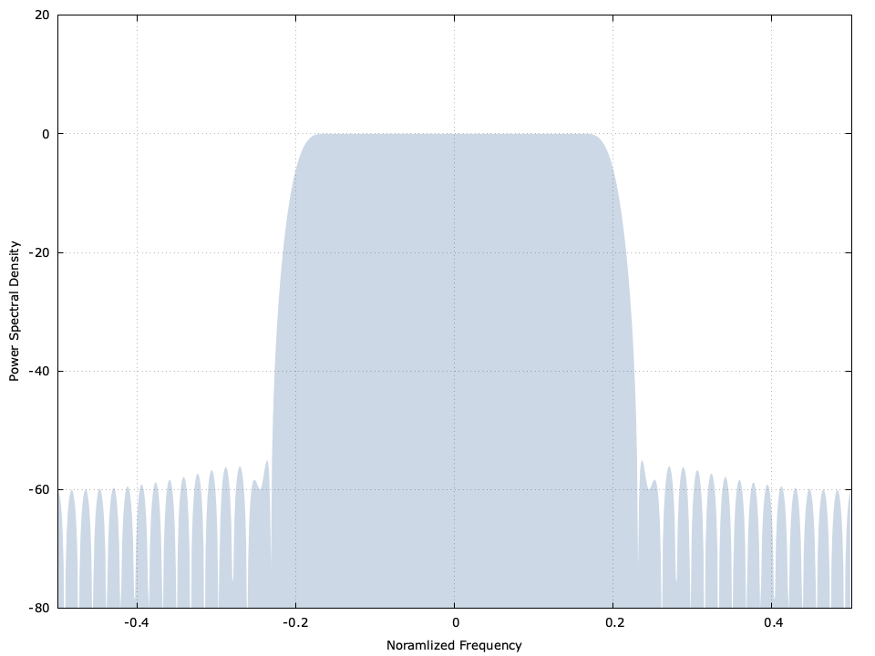
Figure [basic_fir_filter_design]. Basic non-recursive (FIR) filter design response
The goal of designing a non-recursive (finite impulse response) low-pass digital filter is to determine the set of coefficients which provide a frequency response as close to the ideal as possible. While the exact interpretation of that goal may vary based on the application, a general design strategy is to have a filter which has the following three qualities:
- as short a time duration as possible : increasing the time duration increases two undesirable properties of the filter: the computational complexity and the filter delay
- minimize the transition between the passband and stopband : the purpose of the filter is to let some frequencies through while rejecting others. The larger the transition is, the more undesired frequencies sneak through
- maximize attenuation in the stop-band : the more attenuation in the stop-band, the better the filter is at rejecting unwanted signals
There are of course other qualities of a filter for which we could include in our design (pass-band ripple, group delay), but those are topics for another post.
The truth is that these particular qualities are inextricably linked. As a general rule, the longer the filter the sharper its transition and the better it attenuates in the stop-band.
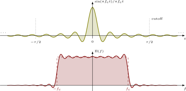
Figure [fig_sinc]. Infinite sinc with corresponding PSD "ideal", truncated sinc and its PSD "practical"
There are many, many options for our windowing function [ref:cite:harris1978] , each one balancing performance in some dimension with the complexity in computing it. The Prolate spheroidal wave series (PSWS) is proven to minimize power outside the main spectral lobe [ref:cite:Slepian] , but is very difficult to compute. While there are some very good approximations to PSWS such as the Kaiser-Bessel window [ref:cite:Kaiser] , there are some very simple smoothing windows which provide performance that is quite acceptable for most applications.
In this tutorial we will use the Hamming window, named after its discoverer, the brilliant mathematician Richard Hamming. The Hamming window is ubiquitous in filter design for its simplicity yet moderate performance.
$$ w_h(t;\tau) = 0.53836 - 0.46164 \cos( 2 \pi t ),\,\,\,-\frac{\tau}{2} \leq t \leq \frac{\tau}{2} $$This provides the resulting spectrum:
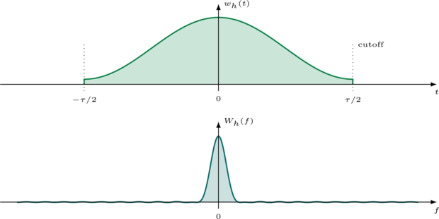
Figure [fig_hamming]. Hamming function with corresponding PSD.
Notice from the above figure how the the main lobe does not have as sharp a cutoff as that of the sinc function, but has sidelobes that are much lower for a signal of the same time duration. By multiplying the sinc together with the smoothing window we get a compromise between sharpness of the filter and stop-band attenuation.
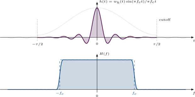
Figure [fig_filter]. Composite response of sinc and Hamming window.
coding it up∞
The source code above is broken up into three sections: filter design, filter analysis, and writing the results to a file for plotting. The filter design follows the description above. A discrete Fourier transform (DFT) is required for frequency analysis. While not nearly as efficient as a fast Fourier transform (FFT), the DFT is simple to program. Finally the resulting power spectral density of the filter is written to a file for plotting.
Compile basic_fir_filter_design.c above and run the program with:
gcc -Wall -O2 -lm -lc -o basic_fir_filter_design.c -o basic_fir_filter_design
./basic_fir_filter_design
...which should produce the following output:
#    frequency     PSD [dB]
   -0.50000000   -60.028615
   -0.49875000   -60.246393
   -0.49750000   -60.921650
   -0.49625000   -62.134442
   -0.49500000   -64.066805
   -0.49375001   -67.148102
   -0.49250001   -72.747444
     ...
    0.00250000     0.003389
    0.00375003     0.003005
    0.00500000     0.002495
    0.00625002     0.001871
    0.00749999     0.001167
     ...
    0.49250001   -72.747444
    0.49374998   -67.145936
    0.49500000   -64.066805
    0.49624997   -62.135224
    0.49750000   -60.921650
    0.49874997   -60.246316
When plotted this gives you the spectrum response at the top of this post.